
In short
405, 488, 561 and around 640 nm cover most routine dye panels. Many systems add 445, 514 or 594 nm.
Specify power at the sample, then work backwards through your own optical path. Measured end to end transmission varies widely between systems.
Power stability and noise decide whether intensities are comparable between images, but the laser is only one contributor.
Confocal microscopes are sold as complete instruments, so the laser inside them rarely gets discussed on its own. That changes when you are building an instrument, replacing a failed source or adding a line to an existing system. Then the laser becomes a component you have to specify, and the numbers that matter are not the ones on the front of the datasheet.
The common laser lines
Commercial dye panels cluster around a small set of excitation lines. Four of them cover a large share of routine work, and most systems offer one or two more for cases where the standard four sit badly on the absorption peak.
| Line | Common fluorophores | Note | From RGB |
|---|---|---|---|
| 405 nm | DAPI, Hoechst, Alexa Fluor 405 | Sits on the shoulder of the DAPI band, not its peak | 405 nm module |
| 445 nm | CFP | Usually excites CFP more efficiently than 405 nm | yes |
| 488 nm | GFP, FITC, Alexa Fluor 488 | The most used single line | yes |
| 514 / 515 nm | YFP | Where YFP and GFP must be separated | yes |
| 561 nm | mCherry, TRITC | DPSS wavelength | no |
| 594 nm | Texas Red, Alexa Fluor 594 | Often a better match than 561 nm | no |
| 633 / 638 / 640 nm | Cy5, Alexa Fluor 647, APC | Close together but not interchangeable with a given filter set | 633 nm module |
Check the actual excitation and emission spectra of your dyes against your dichroics and emission filters before fixing a line. Two wavelengths a few nanometres apart can behave very differently once a filter set is in the path. For how excitation wavelength, Stokes shift and dye choice interact, see which fluorophore needs which line.
Power at the sample, not at the aperture
The number on a laser datasheet is measured at its output. What matters is what arrives at the focal plane, and the path between them loses a lot. The figures below are typical ranges for the individual stages. They are not a specification for any particular instrument.
| Stage | Typical transmission |
|---|---|
| Fiber coupling | 50 to 80 % |
| AOTF or filter wheel | 60 to 90 % |
| Scan head and dichroics | 50 to 80 % |
| Objective | 70 to 90 % |
| Multiplied end to end | roughly 10 to 50 % |
Two traps when you use this
Do not count fiber coupling twice. If the laser is specified at the fiber output, that loss is already inside the number you were given.
Transmission is wavelength dependent. Dichroics, AOTF efficiency and objective coatings all vary across the range. Size the source for the worst relevant line, not for an average.
Worked through: at 10 to 50 % end to end, 1 mW at the sample needs roughly 2 to 10 mW from the source. Add margin for component ageing and for the drop in diode output over service life, and you arrive at a sensible specification of around 5 to 20 mW per line for that target. The honest version of this calculation is to measure the transmission of your own system rather than to inherit a rule of thumb.
As a starting point for the target itself, many confocal applications work in the region of 1 to 10 mW at the sample for point scanning. Treat that as orientation. The real figure depends on sample, objective, detector sensitivity, dwell time and how much bleaching you are prepared to accept.
What the source should deliver
| Parameter | Why it matters | How to specify it |
|---|---|---|
| Power stability | Intensity differences between images become artefacts rather than biology | With a stated period and measurement point. The laser is one contributor among AOTF, fiber and polarization |
| Noise | Appears as pixel noise and forces longer dwell times | Separate fast intensity noise from long term drift, and state the measurement bandwidth |
| Beam quality | Decides how tightly the beam focuses and how well it couples | Ask for M² and the beam mode, not just the label TEM00 |
| Polarization | Polarization sensitive optics in the scan head cause throughput to vary | Specify at the relevant output, after the fiber if there is one |
| Modulation | Blanking during scanner retrace avoids dose that produces no signal | Only needed from the laser if the microscope has no AOTF or AOM doing the job |
That last row is worth a sentence. Most commercial confocal systems already contain an AOTF that handles blanking and intensity control, and its switching time and synchronisation matter more than the laser’s own modulation bandwidth. Direct modulation of the source becomes a requirement mainly in custom builds without such a modulator, which is the usual situation when an OEM laser module goes into a new instrument.
 Built for microscopy
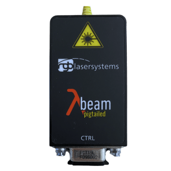
Lambda Beam Pigtailed
Polarization maintaining single mode fiber · temperature stabilized · 405 to 1550 nm
View range
Built for microscopy
Lambda Beam Pigtailed
Polarization maintaining single mode fiber · temperature stabilized · 405 to 1550 nm
View range
Point scanning or spinning disk
| Point scanning | Spinning disk | |
|---|---|---|
| Illumination | one focused spot, sequential | many spots in parallel |
| Total power needed | lower | higher, the factor depends on pinhole count, disk and camera |
| Modulation | retrace blanking is useful | less critical |
| Speed | limited by the scanner | can be considerably faster |
Spinning disk systems spread the same job over many simultaneous foci, so the required total laser power is higher. How much higher is not a fixed multiple: pinhole count, disk design, camera sensitivity, exposure time and the sample all enter. Work it out for the specific head rather than applying a factor.
Why confocal systems are usually fiber coupled
- Reproducible beam geometry. A single mode fiber spatially filters the beam, so what reaches the scan head is similar across units regardless of diode to diode variation.
- Alignment leaves the production line. You align the fiber output into the scan head rather than the laser itself in every unit.
- Thermal separation. The laser and its heat sit away from the optical head.
- Combining lines. Several wavelengths arrive on a common axis instead of each needing its own alignment.
It is not free. Coupling costs optical power, the fiber has to be single mode across every wavelength you send through it, and polarization maintaining fiber adds launch alignment and connector requirements. For multi line systems the benefits usually win. For a single line bench setup, free space may be the simpler answer.
Frequently asked questions
Does a confocal microscope need a laser?
Confocality comes from the geometry: a point focus paired with a pinhole that rejects out-of-focus light. That does not strictly require a laser, and early Nipkow disk instruments used arc lamps. In practice almost all commercial point scanning systems use lasers, because they deliver high brightness into a small, narrowband, well defined focus, which lamps cannot match.
How many laser lines do I need?
One per fluorophore channel you want to separate cleanly. Four lines around 405, 488, 561 and 640 nm cover many commercial panels. Add 445 nm for CFP or 594 nm for the Texas Red family if those appear in your work. Specialised instruments often manage with one or two.
How much laser power does confocal microscopy need?
For point scanning, often in the region of 1 to 10 mW at the sample, with large variation by application. Because the optical path typically transmits only 10 to 50 %, the source is usually specified several times higher per line. Measure your own path rather than relying on a general figure.
Can I add a wavelength to an existing microscope?
Often yes, if the system has a free fiber input and the dichroics and emission filters pass the new band. The laser is usually the easy part. Check the filter set first.
What are the downsides of confocal laser scanning?
Point scanning builds the image sequentially and is therefore slower than widefield. Spinning disk architectures scan in parallel and can be fast enough for live cell work. Concentrating the dose into a scanned focus tends to increase photobleaching and phototoxicity, though the outcome depends on total dose, scan strategy, frame rate and the sample rather than on the architecture alone.
Building or upgrading a confocal system?
Tell us the lines you need, the power required at the sample and your fiber format. We will work back through the loss budget with you and say which numbers need measuring rather than assuming.